
TargetDiff
TargetDiff 概述
TargetDiff 在干什么
TargetDiff是一种基于三维等变扩散模型的分子生成工具,专注于目标蛋白感知的分子设计和结合亲和力预测,旨在加速药物发现进程。其核心应用包括:
靶向分子生成:根据目标蛋白的三维结合口袋结构,生成与之空间匹配且具有高结合亲和力的候选分子(例如小分子配体)
结合亲和力预测:通过无监督特征提取,提供分子与靶点蛋白的结合强度估计,辅助药物筛选
分子结构优化:生成具有合理三维构象的分子,避免传统方法(如自回归模型)因逐步生成导致的几何失真问题
TargetDiff 解决的问题
| 🚀 问题类别 | ❌ 传统方法的局限 | ✅ TargetDiff 的解决方案 |
|---|---|---|
| 几何约束建模不足 | 🚨 基于体素化密度或自回归采样,常生成不合理的键长、键角,刚性片段(如苯环)易扭曲,结构失真 | ✨ 采用 SE(3)-等变扩散模型,保证生成结构在旋转/平移下几何一致,自动对齐结合位点,避免失真 |
| 三维等变性缺失 | 🚨 忽略分子与靶点之间的相对空间关系,生成构象与蛋白结合口袋匹配性差 | ✨ 利用 等变神经网络 建模,天然保持三维旋转、平移等变性,提高结合构象的空间合理性 |
| 标注数据依赖性强 | 🚨 亲和力预测依赖大量标注数据,数据昂贵且难以获取 | ✨ 通过 无监督学习提取分子-靶点复合物的隐含表示,降低对监督数据依赖 |
| 生成效率低下 | 🚨 自回归方法需逐步生成原子,随分子尺寸增长时间成本快速上升 | ✨ 扩散模型并行生成所有原子,显著提升大分子生成效率 |
| 位置与类型分离生成 | 🚨 原子位置与类型分离生成,可能导致物理结构不一致 | ✨ 通过 联合生成坐标与类型 的扩散流程,同时优化结构和类型,增强物理合理性 |
| 功能单一,泛化弱 | 🚨 大多数模型仅用于生成或预测,特征泛化能力弱 | ✨ TargetDiff 同时作为 分子生成器 + 无监督特征提取器,用于结合亲和力排名与预测,效果超越EGNN |
| 评估标准不全面 | 🚨 传统评估指标如 RMSD 或 Tanimoto 不能全面反映三维构象质量 | ✨ 引入 刚性片段一致性 RMSD 和 键距 JS 散度 等新指标,更好量化结构真实性与物理合理性 |
TargetDiff 尚未解决的问题
化学键生成的依赖性: 当前模型依赖后处理工具(如OpenBabel)推断化学键,可能引入误差。未来需将键生成直接纳入扩散过程
可合成性与药物相似性不足: 在QED(药物相似性)和SA(可合成性)评分上落后于Pocket2Mol,需通过 片段生成技术优化分子子结构
立体冲突问题: 生成的分子可能 因原子间距过近导致立体冲突(clash),需 引入最小距离约束或后处理优化
采样速度与精度权衡: 原始DDPM采样需1000步,虽可通过DPM-Solver++加速至10步,但可能牺牲结合亲和力;需进一步优化采样算法
多目标优化挑战: 在同时优化结合亲和力、药物相似性和多样性时存在权衡(如ALIDIFF实验显示低 值增强亲和力但降低 QED)
TargetDiff 理论
TargetDiff 原理简述
生成模型
- 学习一个分布 distribution —— 如何学习?
- 已知一个简单的分布(高斯分布、均匀分布...),从中采样(sample)
- 利用 将简单分布映射到一个复杂分布
- 生成样本 , 近似于复杂分布(我们无法从复杂分布中直接采样)
- 利用学习到的分布,从中采样得到结果
DDPM
Denoising Diffusion Probabilistic Models 去噪扩散概率模型
核心思想
- 前向扩散过程(Forward Diffusion Process)
- 逐步加噪,记录噪声和中间产物,训练网络预测噪声
- 反向去噪过程(Reverse Denoising Process)
- 从纯噪声开始,逐步去噪,恢复出想要的目标数据
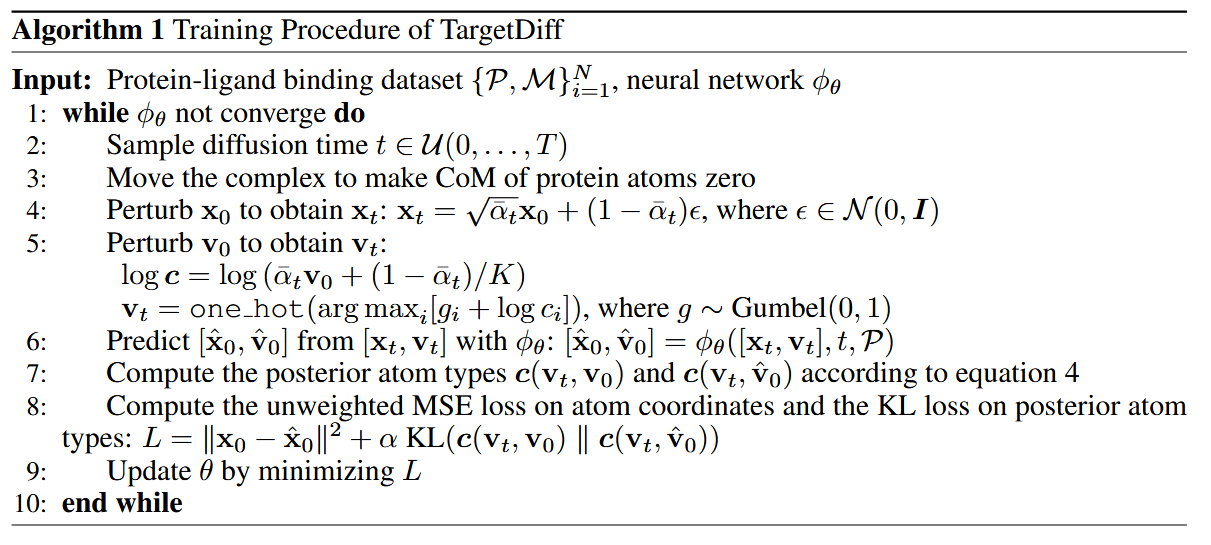
TargetDiff 训练算法流程
输入:蛋白质-配体的结合数据集
扩散条件初始化:采样时间步 —— 从均匀分布 中采样扩散时间
预处理:将蛋白质原子的质心移动到原点,以对齐配体和蛋白质的位置,确保数据在空间上的一致性
加噪:网络中主要是针对 位置 和 原子类型 进行扰动,逐步加噪
- ,其中 是从正态分布 中采样的噪声
预测: ,预测扰动位置和类型,即 和 ,条件是当前的 、、时间步 和蛋白质信息
计算后验类型分布:根据公式计算原子类型的后验分布 和
损失函数:
- 均方误差 MSE:度量原子坐标的偏差
- KL 散度(KL-divergence):度量类型分布的差异
更新参数: 最小化损失函数 来更新模型参数
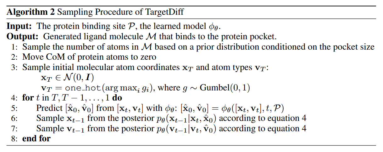
TargetDiff 采样算法流程
输入:蛋白质结合位点(binding site) 与 训练好的模型
输出:由模型生成的能与蛋白质口袋结合的配体分子
确定原子数量:基于口袋大小,从一个先验分布中采样一个生成的配体分子的原子数量
预处理:移动蛋白质原子的质心至坐标原点,使位置标准化,以确保生成的配体与蛋白质结合位点对齐
初始化:采样一个初始的原子坐标(coordinates) 和 原子类型
- —— 从标准正态分布 中采样
- (反向去噪)
预测: ,预测扰动位置和类型,即 和 ,条件是当前的 、、时间步 和蛋白质信息
根据后验分布 对原子位置 进行采样
根据后验分布 对原子类型 进行采样
TargetDiff 代码
代码解读
Velvet0314/targetdiff at 4LearnOnly
环境安装 Tips
- 推荐在 Linux 下进行环境安装(可以用 WSL) —— Vina 需要 Linux 环境
- 注意 Pytorch, Cuda, Python 的版本对应
- 需要安装对应版本的 cudatoolkit 实现 Pytorch 中利用 cuda 进行 GPU 的加速
- 我的环境在
myenvironment.yaml中,可以跑通
额外内容
- test_cuda.py 用于测试 cuda 是否启用
- viewlmdb.py 用于可视化输入数据
训练流程
主要代码在 train_diffusion.py和molopt_score_model.py中
解析命令行 —— 训练的超参数的设置
数据的预处理 —— 数据输入的预处理
- 主要是进行数据的映射与反映射
数据集处理 —— 数据加载与划分
初始化模型 —— 调用
molopt_score_model.py中的模型训练 —— 关键在
model.get_diffusion_loss函数中- 生成时间步 —— 算法step2
# sample noise levels if time_step is None: time_step, pt = self.sample_time(num_graphs, protein_pos.device, self.sample_time_method) else: pt = torch.ones_like(time_step).float() / self.num_timesteps a = self.alphas_cumprod.index_select(0, time_step) # (num_graphs, ) - 质心归零 —— 算法step3
protein_pos, ligand_pos, _ = center_pos( protein_pos, ligand_pos, batch_protein, batch_ligand, mode=self.center_pos_mode) - 对 原子位置 pos & 原子类型 v 进行加噪 —— 算法step4&5
# perturb pos and v a_pos = a[batch_ligand].unsqueeze(-1) # (num_ligand_atoms, 1) pos_noise = torch.zeros_like(ligand_pos) pos_noise.normal_() # Xt = a.sqrt() * X0 + (1-a).sqrt() * eps ligand_pos_perturbed = a_pos.sqrt() * ligand_pos + (1.0 - a_pos).sqrt() * pos_noise # pos_noise * std # Vt = a * V0 + (1-a) / K log_ligand_v0 = index_to_log_onehot(ligand_v, self.num_classes) ligand_v_perturbed, log_ligand_vt = self.q_v_sample(log_ligand_v0, time_step, batch_ligand) - 前向传播计算,得到每阶段加噪的结果和网络预测的噪声 —— 算法step6
# forward-pass NN, feed perturbed pos and v, output noise preds = self( protein_pos=protein_pos, protein_v=protein_v, batch_protein=batch_protein, init_ligand_pos=ligand_pos_perturbed, init_ligand_v=ligand_v_perturbed, batch_ligand=batch_ligand, time_step=time_step ) pred_ligand_pos, pred_ligand_v = preds['pred_ligand_pos'], preds['pred_ligand_v'] # 网络预测的噪声 pred_pos_noise = pred_ligand_pos - ligand_pos_perturbed # atom position if self.model_mean_type == 'noise': pos0_from_e = self._predict_x0_from_eps( xt=ligand_pos_perturbed, eps=pred_pos_noise, t=time_step, batch=batch_ligand) pos_model_mean = self.q_pos_posterior( x0=pos0_from_e, xt=ligand_pos_perturbed, t=time_step, batch=batch_ligand) elif self.model_mean_type == 'C0': pos_model_mean = self.q_pos_posterior( x0=pred_ligand_pos, xt=ligand_pos_perturbed, t=time_step, batch=batch_ligand) else: raise ValueError - 计算后验分布与误差 —— 算法step7&8
# atom pos loss
if self.model_mean_type == 'C0':
	target, pred = ligand_pos, pred_ligand_pos
elif self.model_mean_type == 'noise':
	target, pred = pos_noise, pred_pos_noise
else:
	raise ValueError

loss_pos = scatter_mean(((pred - target) ** 2).sum(-1), batch_ligand, dim=0)
loss_pos = torch.mean(loss_pos)

# atom type loss
log_ligand_v_recon = F.log_softmax(pred_ligand_v, dim=-1)
log_v_model_prob = self.q_v_posterior(log_ligand_v_recon, log_ligand_vt, time_step, batch_ligand)
log_v_true_prob = self.q_v_posterior(log_ligand_v0, log_ligand_vt, time_step, batch_ligand)
kl_v = self.compute_v_Lt(log_v_model_prob=log_v_model_prob, log_v0=log_ligand_v0,
	log_v_true_prob=log_v_true_prob, t=time_step, batch=batch_ligand)

loss_v = torch.mean(kl_v)
loss = loss_pos + loss_v * self.loss_v_weight
- 生成时间步 —— 算法step2
采样流程
主要代码在 sample_diffusion.py和molopt_score_model.py中
解析命令行 —— 采样的超参数的设置
加载训练好的模型 —— ckpt -> checkpoint
数据的预处理 —— 采用和模型训练时的相同的处理(所有的 config 均来自于选取的模型的训练时的配置)
初始化模型 —— 调用
molopt_score_model.py中的模型采样 —— 关键在
sample_diffusion_ligand函数 和model.sample_diffusion函数中- 确定原子数量 —— 算法step1
# 步骤一:确定原子数量 # 这里有三种方式,其中第一种对应算法中的步骤 if sample_num_atoms == 'prior': # 根据先验分布采样配体原子数量 pocket_size = atom_num.get_space_size(data.protein_pos.detach().cpu().numpy()) # 计算口袋大小 ligand_num_atoms = [atom_num.sample_atom_num(pocket_size).astype(int) for _ in range(n_data)] # 采样原子数量 batch_ligand = torch.repeat_interleave(torch.arange(n_data), torch.tensor(ligand_num_atoms)).to(device) # 生成配体批次索引 elif sample_num_atoms == 'range': # 按顺序指定配体原子数量 ligand_num_atoms = list(range(current_i + 1, current_i + n_data + 1)) # 生成原子数量列表 batch_ligand = torch.repeat_interleave(torch.arange(n_data), torch.tensor(ligand_num_atoms)).to(device) # 生成配体批次索引 elif sample_num_atoms == 'ref': # 使用参考数据的原子数量 batch_ligand = batch.ligand_element_batch # 获取配体的批次索引 ligand_num_atoms = scatter_sum(torch.ones_like(batch_ligand), batch_ligand, dim=0).tolist() # 计算每个样本的原子数量 else: raise ValueError # 抛出异常 - 质心归零 —— 算法step2
# 步骤二:初始化配体位置 center_pos = scatter_mean(batch.protein_pos, batch_protein, dim=0) # 计算每个蛋白质的中心位置 batch_center_pos = center_pos[batch_ligand] # 获取每个配体原子的中心位置 ... protein_pos, init_ligand_pos, offset = center_pos( protein_pos, init_ligand_pos, batch_protein, batch_ligand, mode=center_pos_mode) - 采样初始化 —— 算法step3
# 步骤三:采样初始化——原子位置 init_ligand_pos = batch_center_pos + torch.randn_like(batch_center_pos) # 添加随机噪声,初始化配体位置 # 步骤三:采样初始化—原子类型 if pos_only: # 如果仅采样位置,使用初始的配体特征 init_ligand_v = batch.ligand_atom_feature_full else: # 否则,从均匀分布中采样初始v值 # 算法中对应的步骤 uniform_logits = torch.zeros(len(batch_ligand), model.num_classes).to(device) # 创建均匀分布的logits init_ligand_v = log_sample_categorical(uniform_logits) # 采样v值 - 反转时间步 —— 算法step4
# time sequence # 反转时间步,从 T-1 到 0 time_seq = list(reversed(range(self.num_timesteps - num_steps, self.num_timesteps))) - 预测 —— 算法step5
# 步骤五:从时间步 T 开始使用模型 ϕ₀ 从 [xₜ, vₜ] 预测 [x̂₀, v̂₀] # self() 调用前向传播 forward() preds = self( protein_pos=protein_pos, protein_v=protein_v, batch_protein=batch_protein, init_ligand_pos=ligand_pos, init_ligand_v=ligand_v, batch_ligand=batch_ligand, time_step=t ) # Compute posterior mean and variance if self.model_mean_type == 'noise': pred_pos_noise = preds['pred_ligand_pos'] - ligand_pos pos0_from_e = self._predict_x0_from_eps(xt=ligand_pos, eps=pred_pos_noise, t=t, batch=batch_ligand) v0_from_e = preds['pred_ligand_v'] elif self.model_mean_type == 'C0' pos0_from_e = preds['pred_ligand_pos'] v0_from_e = preds['pred_ligand_v'] else: raise ValueError - 采样下一时间步的 原子位置 与 原子类型 —— 算法step6&7
# 步骤六&七:由后验分布采样 [xₜ₋₁, vₜ₋₁]
pos_model_mean = self.q_pos_posterior(x0=pos0_from_e, xt=ligand_pos, t=t, batch=batch_ligand)
pos_log_variance = extract(self.posterior_logvar, t, batch_ligand)

# no noise when t == 0
nonzero_mask = (1 - (t == 0).float())[batch_ligand].unsqueeze(-1)
ligand_pos_next = pos_model_mean + nonzero_mask * (0.5 * pos_log_variance).exp() * torch.randn_like(ligand_pos)
ligand_pos = ligand_pos_next

# 若不只是采样位置,则采样原子类型 vₜ₋₁
if not pos_only:
	log_ligand_v_recon = F.log_softmax(v0_from_e, dim=-1)
	log_ligand_v = index_to_log_onehot(ligand_v, self.num_classes)
	log_model_prob = self.q_v_posterior(log_ligand_v_recon, log_ligand_v, t, batch_ligand)
	ligand_v_next = log_sample_categorical(log_model_prob)

	v0_pred_traj.append(log_ligand_v_recon.clone().cpu())
	vt_pred_traj.append(log_model_prob.clone().cpu())
	ligand_v = ligand_v_next

ori_ligand_pos = ligand_pos + offset[batch_ligand]
pos_traj.append(ori_ligand_pos.clone().cpu())
v_traj.append(ligand_v.clone().cpu())
- 确定原子数量 —— 算法step1
评估流程
主要在evaluate_diffusion.py 和 evaluate_from_meta.py 中
评估流程整体上就是对一些指标进行计算来衡量生成分子的好坏
Jensen-Shannon divergence between the distributions of bond distance
主要在 eval_bond_length.py 中
def bond_distance_from_mol(mol):
	   pos = mol.GetConformer().GetPositions()
	pdist = pos[None, :] - pos[:, None]
	pdist = np.sqrt(np.sum(pdist ** 2, axis=-1))
	all_distances = []

	for bond in mol.GetBonds():
		s_sym = bond.GetBeginAtom().GetAtomicNum()
		e_sym = bond.GetEndAtom().GetAtomicNum()
		s_idx, e_idx = bond.GetBeginAtomIdx(), bond.GetEndAtomIdx()
		bond_type = utils_data.BOND_TYPES[bond.GetBondType()]
		distance = pdist[s_idx, e_idx]
		all_distances.append(((s_sym, e_sym, bond_type), distance))
	return all_distances
Distribution for distances of all atom and carbon-carbon pairs
主要在 eval_bond_length.py 中
c_bond_length_profile = eval_bond_length.get_bond_length_profile(all_bond_dist)
c_bond_length_dict = eval_bond_length.eval_bond_length_profile(c_bond_length_profile)
logger.info('JS bond distances of complete mols: ')
print_dict(c_bond_length_dict, logger)

success_pair_length_profile = eval_bond_length.get_pair_length_profile(success_pair_dist)

success_js_metrics = eval_bond_length.eval_pair_length_profile(success_pair_length_profile)
print_dict(success_js_metrics, logger)

atom_type_js = eval_atom_type.eval_atom_type_distribution(success_atom_types)
logger.info('Atom type JS: %.4f' % atom_type_js)
...
def eval_bond_length_profile(bond_length_profile: BondLengthProfile) -> Dict[str, Optional[float]]:
	metrics = {}

	# Jensen-Shannon distances
	for bond_type, gt_distribution in eval_bond_length_config.EMPIRICAL_DISTRIBUTIONS.items():
		if bond_type not in bond_length_profile:
			metrics[f'JSD_{_bond_type_str(bond_type)}'] = None
		else:
			metrics[f'JSD_{_bond_type_str(bond_type)}'] = sci_spatial.distance.jensenshannon(gt_distribution,                                                bond_length_profile[bond_type])
	return metrics

def eval_pair_length_profile(pair_length_profile):
	metrics = {}

	for k, gt_distribution in eval_bond_length_config.PAIR_EMPIRICAL_DISTRIBUTIONS.items():
		if k not in pair_length_profile:
			metrics[f'JSD_{k}'] = None
		else:
			metrics[f'JSD_{k}'] = sci_spatial.distance.jensenshannon(gt_distribution, pair_length_profile[k])
	return metrics

def eval_atom_type_distribution(pred_counter: Counter):
	total_num_atoms = sum(pred_counter.values())
	pred_atom_distribution = {}
	for k in ATOM_TYPE_DISTRIBUTION:
		pred_atom_distribution[k] = pred_counter[k] / total_num_atoms
	# print('pred atom distribution: ', pred_atom_distribution)
	# print('ref  atom distribution: ', ATOM_TYPE_DISTRIBUTION)
	js = sci_spatial.distance.jensenshannon(np.array(list(ATOM_TYPE_DISTRIBUTION.values())),
												np.array(list(pred_atom_distribution.values())))
	return js
Percentage of different ring sizes
主要在 evaluate_diffusion.py 中
def print_ring_ratio(all_ring_sizes, logger):
	for ring_size in range(3, 10):
		n_mol = 0
		for counter in all_ring_sizes:
			if ring_size in counter:
				n_mol += 1
		logger.info(f'ring size: {ring_size} ratio: {n_mol / len(all_ring_sizes):.3f}')

# check ring distribution
print_ring_ratio([r['chem_results']['ring_size'] for r in results], logger)
High Affinity
主要在 docking_vina.py. 和 docking_qvina.py 中
docking_mode 的选择
evaluation_from_meta.pydocking_mode是默认的vina_full模式:parser.add_argument('--docking_mode', type=str, default='vina_full', choices=['none', 'qvina', 'vina', 'vina_full', 'vina_score'])evaluation_diffusion.py取决于命令行里的参数:parser.add_argument('--docking_mode', type=str, default='vina_full', choices=['qvina', 'vina_score', 'vina_dock', 'none'])参考的命令行:
python scripts/evaluate_diffusion.py {OUTPUT_DIR} --docking_mode vina_score --protein_root data/test_set
Affinity 的计算
def run(self, mode='dock', exhaustiveness=8, **kwargs):

  	ligand_pdbqt = self.ligand_path[:-4] + '.pdbqt'
  	protein_pqr = self.receptor_path[:-4] + '.pqr'
  	protein_pdbqt = self.receptor_path[:-4] + '.pdbqt'

  	lig = PrepLig(self.ligand_path, 'sdf')
  	lig.get_pdbqt(ligand_pdbqt)

  	prot = PrepProt(self.receptor_path)

  	if not os.path.exists(protein_pqr):
  		prot.addH(protein_pqr)

  	if not os.path.exists(protein_pdbqt):
  		prot.get_pdbqt(protein_pdbqt)

  	dock = VinaDock(ligand_pdbqt, protein_pdbqt)
  	dock.pocket_center, dock.box_size = self.center, [self.size_x, self.size_y, self.size_z]
  	score, pose = dock.dock(score_func='vina', mode=mode, exhaustiveness=exhaustiveness, save_pose=True, **kwargs)
  	return [{'affinity': score, 'pose': pose}]
Diversity
TargetDiff 中无该部分代码,但是单独给出一个用于计算 Diversity 的标准代码
def tanimoto_sim(mol, ref):
	fp1 = Chem.RDKFingerprint(ref)
	fp2 = Chem.RDKFingerprint(mol)
	return DataStructs.TanimotoSimilarity(fp1,fp2)

def calc_pairwise_sim(mols):
	n = len(mols)
	sims = []
	 for i in range(n):
		for j in range(i + 1, n):
			sims.append(tanimoto_sim(mols[i], mols[j]))
	return np.array(sims)

def computer_diversity(mols):
	div_all = []
	# for result in tqdm(results):
	div_all.append(np.mean(1 - calc_pairwise_sim(mols)))
	div_all = np.array(div_all)
	div_all = div_all[~np.isnan(div_all)]
	return div_all
...
for ligand_filename, smiles_list in protein_ligand_dict.items():
	diversity = computer_diversity(smiles_list)
	protein_diversities.append(diversity)
	print(f"{ligand_filename} 的diversity: {diversity}")
print(len(protein_ligand_dict))

mean_diversity = np.mean(protein_diversities)
median_diversity = np.median(protein_diversities)